3D Gaussian Splatting, Explained

I keep running into Gaussian splatting — in mapping demos, in VR captures, in the "scan your living room with your phone" apps — and for a while I only had a fuzzy sense of what it actually was. So I sat down to understand it properly, and this post is the explanation I wish I'd had: what problem it solves, how it relates to NeRF, and why it took over so fast. I've built a few interactive pieces along the way so you can poke at the ideas directly.

But first, the payoff — so you know what we're chasing. This is a real scene, captured on an ordinary camera and turned into a Gaussian splat you can fly through in real time. It looks like video, but it's a 3D reconstruction: every frame is rendered live from a viewpoint no photo was ever taken from.

A 3D Gaussian splatting fly-through of a real scene (via @ValigurskyM)

That smooth, photorealistic fly-through from a handful of ordinary photos is the goal. The rest of this post is how you get there.

The problem both NeRF and splatting are trying to solve

Start with the goal, because NeRF and Gaussian splatting are two answers to the same question: novel-view synthesis. You have a handful of photos of a scene, and you know roughly where each camera was. Now render the scene from a viewpoint that no photo was ever taken from — smoothly, photorealistically, as if you'd had a camera there the whole time.

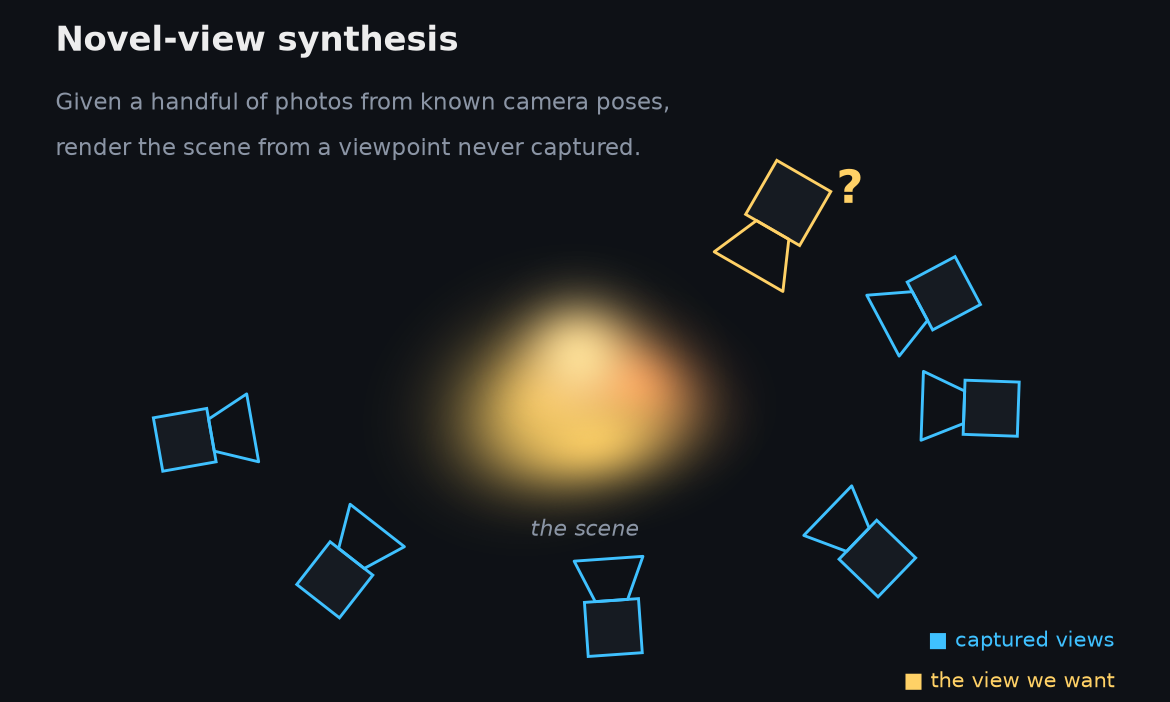
This is harder than it sounds. Stitching photos into a panorama doesn't work — you're not rotating in place, you're moving through the scene, so everything shifts with parallax. You have to recover something about the 3D structure to fill in the views in between. Classical photogrammetry does this by building an explicit mesh: find surfaces, triangulate them, paint textures on top. That's great for clean, well-defined objects and miserable for leaves, hair, wires, smoke, and glass. The interesting work of the last few years is about representations that don't need you to commit to a mesh up front.

How NeRF does it

NeRF (2020) had a beautifully simple idea: make the scene a function. Train a small neural network that takes a 3D point and a viewing direction — five numbers, (x, y, z, θ, φ) — and returns the color and the density at that point. The whole scene lives in the network's weights.

To render a pixel, you shoot a ray out through it and march along the ray, querying the network at many sample points, then integrate color weighted by density and how much light survives to reach the camera. Do that for every pixel and you get an image.

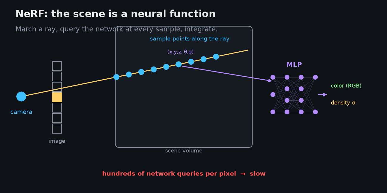
It works astonishingly well. It also has one structural problem baked right into that picture: rendering a single pixel means hundreds of neural-network queries. A full image is millions of pixels. Early NeRFs took days to train and many seconds to render one frame. The representation is elegant — a continuous function over all of space — but it's implicit: nothing about the scene is laid out where you can touch it. Everything has to be re-derived, ray by ray, query by query.

Why Gaussian splatting was invented

Gaussian splatting is, at heart, NeRF made practical for real-time rendering. It keeps the differentiable-rendering idea — optimize a representation until its rendered views match the photos — and throws out the slow part.

Instead of asking a neural network "what's at this 3D point?", 3D Gaussian splatting represents the scene as millions of little soft translucent ellipsoids floating in space. Each ellipsoid is a splat. To render a new view you project the ellipsoids onto the image plane, blend them front-to-back, and read off a photorealistic image. No ray marching, no per-pixel network — just projecting and compositing primitives, which is exactly what GPUs are built to do.

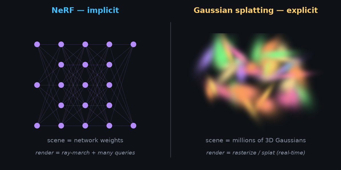
That's the whole shift in one line: NeRF is implicit, splatting is explicit. The 2023 paper made the claim that landed it everywhere — high-quality novel views at real-time 1080p, from an explicit set of 3D Gaussians, optimized directly from calibrated photos with a fast visibility-aware rasterizer.

The mental model I find useful is three ways to reconstruct a room from photos:

• Photogrammetry says: find surfaces, build a mesh, texture it.
• NeRF says: train a neural field mapping location + direction → color + density.
• Gaussian splatting says: fill the scene with soft colored blobs, then nudge their position, shape, opacity, and color until the rendered views match the photos.

What one Gaussian actually is

A single Gaussian is a tiny fuzzy volumetric particle, and it carries only a few numbers:

position:  x, y, z                    — where it sits in space
shape:     a 3D covariance            — encoded as scale + rotation
opacity:   α                          — how solid it is
color:     spherical-harmonic coeffs  — so color can shift with viewing angle

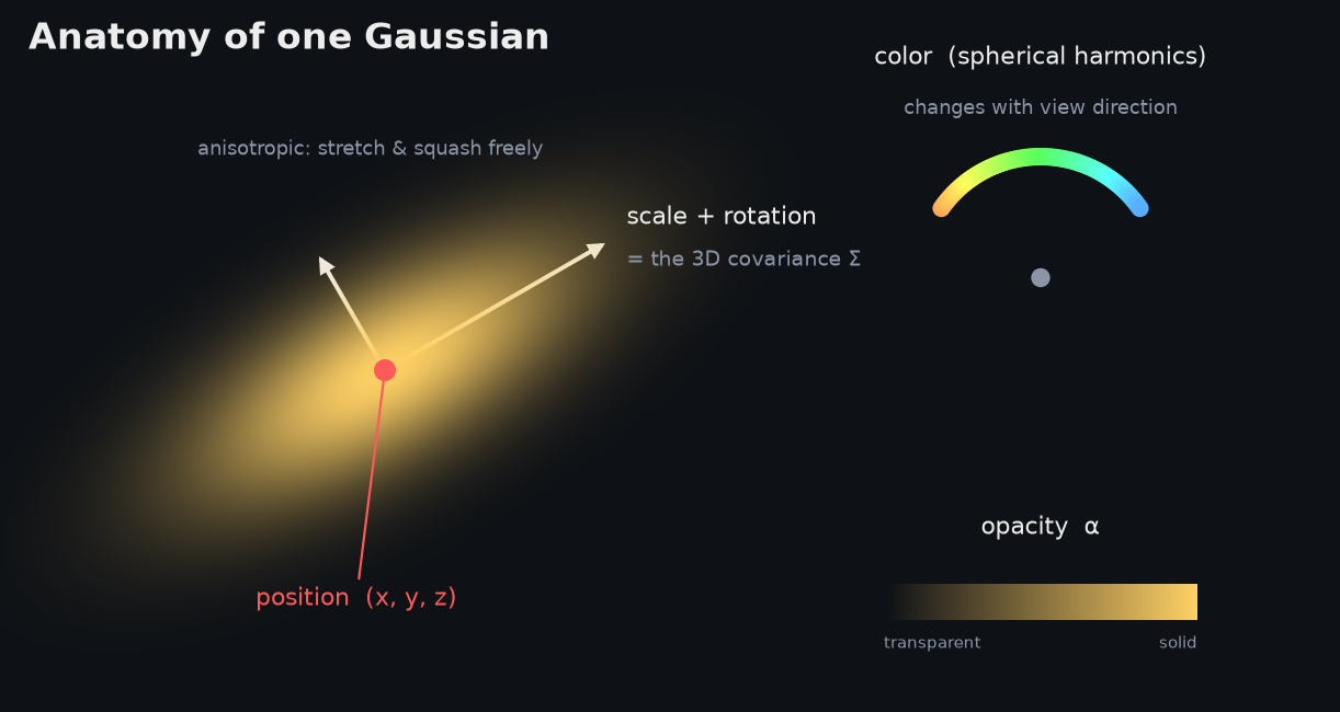
The covariance is the interesting part. A Gaussian isn't a sphere — it's an anisotropic ellipsoid that can be stretched, flattened, and rotated freely. That flexibility is why a million of them can approximate surfaces, thin structures, vegetation, and soft semi-transparent stuff so well: a flat surface becomes a sheet of thin pancake-shaped Gaussians, while a fuzzy region gets fatter, more volumetric ones. The spherical harmonics let a splat look gold from one angle and white from another, which is how you get specular-ish highlights without modeling any real physics.

Here's the thing that took me a moment to internalize: none of this is a neural network in the usual sense. There's no MLP. The "model" is just a giant list of blobs and their parameters. Below is a scene built entirely out of Gaussians — orbit it, and switch between seeing them as soft splats, as the raw ellipsoids, or as bare centers. The same blobs that look like a smooth surface when splatted are, up close, a discrete cloud of oriented lozenges:

Drop the opacity and the surface dissolves into a translucent fog of overlapping blobs — which is what the representation actually is. Crank it back up and your eye reassembles a solid object. That tension between "discrete particles" and "continuous surface" is the whole trick.

How training works

You don't author those millions of Gaussians by hand — you optimize them. The pipeline goes:

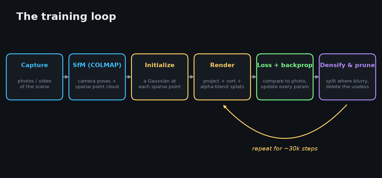
1. Capture many images, or a video. Coverage matters more than count: move around the object, get parallax, avoid motion blur.
2. Estimate camera poses. This is usually COLMAP doing structure-from-motion, which hands you the camera intrinsics, the camera poses, and a sparse 3D point cloud as a by-product.
3. Initialize Gaussians by dropping one at each of those sparse points, with some starting scale, rotation, opacity, and color.
4. Render a training view differentiably: project every visible Gaussian into the image, turn each into a 2D ellipse, sort by depth, alpha-blend, get an image.
5. Compute the loss against the real photo — a photometric term plus an SSIM-style image-similarity term — and backpropagate into the splats. Gradient descent updates every Gaussian's position, scale, rotation, opacity, and color coefficients. You're not training a network; you're optimizing a cloud of differentiable, renderable primitives.
6. Densify and prune. Periodically, the optimizer splits or clones Gaussians in regions that are still blurry, and deletes the ones that have gone nearly transparent or contribute nothing. This interleaved density control — together with the anisotropic covariance — was one of the core tricks of the original method.

Roughly:

gaussians = initialize_from_sparse_sfm_points()

for step in range(training_steps):
    camera, target_image = sample_training_view()
    rendered = render_gaussians(gaussians, camera)
    loss = image_loss(rendered, target_image)
    loss.backward()
    optimizer.step()

    if step % densify_interval == 0:
        split_or_clone_high_error_gaussians()
        prune_low_opacity_or_useless_gaussians()

The loss: what "match the photo" means

Step 5 hides the only real objective in the whole method, so it's worth writing down. Because the renderer is differentiable, I can state exactly what we minimize.

The forward render for a pixel $p$ is alpha compositing — the same front-to-back "over" operator as any graphics pipeline. Take the Gaussians that cover $p$, sort them by depth, and accumulate:

$$C(p) = \sum_i c_i\,\alpha_i(p) \prod_{j<i}\bigl(1-\alpha_j(p)\bigr)$$ $$\alpha_i(p) = o_i\,\exp\!\Bigl(-\tfrac{1}{2}\,(p-\mu_i)^{\top}\,{\Sigma_i'}^{-1}\,(p-\mu_i)\Bigr)$$

Here $c_i$ is the splat's (view-dependent) color, $o_i$ its opacity, and $\mu_i$, $\Sigma_i'$ the center and $2\times2$ covariance of its projected 2D ellipse. The exponential is the Gaussian falloff — a pixel near the center of the ellipse gets nearly full $\alpha$, the edges almost none. The product term is the transmittance: how much light still gets through after the splats in front have taken their cut. Closer, more opaque splats dominate, and once transmittance reaches zero the rest of the list behind is invisible.

The loss then compares that rendered image $C$ against the ground-truth photo $\hat{C}$. The 3DGS paper blends a pixel-wise term with a structural one:

$$\mathcal{L} = (1-\lambda)\,\mathcal{L}_1 + \lambda\,\mathcal{L}_{\text{D-SSIM}}, \qquad \lambda \approx 0.2$$ $$\mathcal{L}_1 = \frac{1}{N}\sum_p \bigl|\,C(p)-\hat{C}(p)\,\bigr|$$ $$\mathcal{L}_{\text{D-SSIM}} = 1 - \mathrm{SSIM}(C,\hat{C})$$

Why two terms? $\mathcal{L}_1$ pulls every pixel toward the right color, but on its own it tolerates a soft, slightly-blurry answer that's "close enough" on average. D-SSIM is built from SSIM, which compares local means, variances, and covariances over small windows — luminance, contrast, and structure — so it specifically punishes the blur and washed-out texture that $\mathcal{L}_1$ shrugs off. Writing it as $1-\mathrm{SSIM}$ makes it zero when the images are identical, so both terms pull the same way.

Everything feeding $C$ — positions, covariances, opacities, color coefficients — is differentiable, so $\partial\mathcal{L}/\partial(\text{each parameter})$ flows back through the compositing and the projection, and one gradient step nudges all of them at once.

Watching it happen is the part that made it click for me. Here's the loop running against a target image: it starts from a sparse scattering of blobs, and as it renders, measures the error, and densifies where things are still vague, the scene sharpens into focus:

This is a real — if miniature — 2D Gaussian-splatting run: a couple of thousand Gaussians optimized by Adam on exactly the L1 + D-SSIM loss above, rendered with the front-to-back compositing equation above, and grown by the same gradient-driven clone / split / prune. Full 3DGS is this same loop in 3D, with view-dependent color and the tile rasterizer. The source is in the repo.

How the GPU makes it real-time

The "real-time 1080p" claim is the whole reason splatting took off, and it falls out of the fact that both halves of the method — drawing a frame and learning the scene — are now rasterization: project primitives, sort them, blend them, instead of NeRF's ray-marching with a network query at every sample. That maps onto a GPU almost perfectly, and the quiet hero of the 2023 paper is the tile-based differentiable rasterizer that does it. Rendering is the forward pass; training wraps that same forward pass in a matching backward pass, so I'll take rendering first.

Rendering on the GPU

A frame is drawn in four GPU stages, and nothing in the loop touches a neural network:

1. Project & cull — one thread per Gaussian. Every Gaussian gets its own GPU thread that frustum-culls it if it's off-screen, projects its 3D mean to a pixel location, and turns its 3D covariance $\Sigma$ into a 2D screen-space covariance $\Sigma' = J\,W\,\Sigma\,W^{\top}J^{\top}$ — $W$ the viewing transform, $J$ the Jacobian of the projection (the "EWA surface-splatting" formula). The same thread evaluates the spherical-harmonic color for the current view direction and computes a screen bounding box from the splat's ~$3\sigma$ radius.
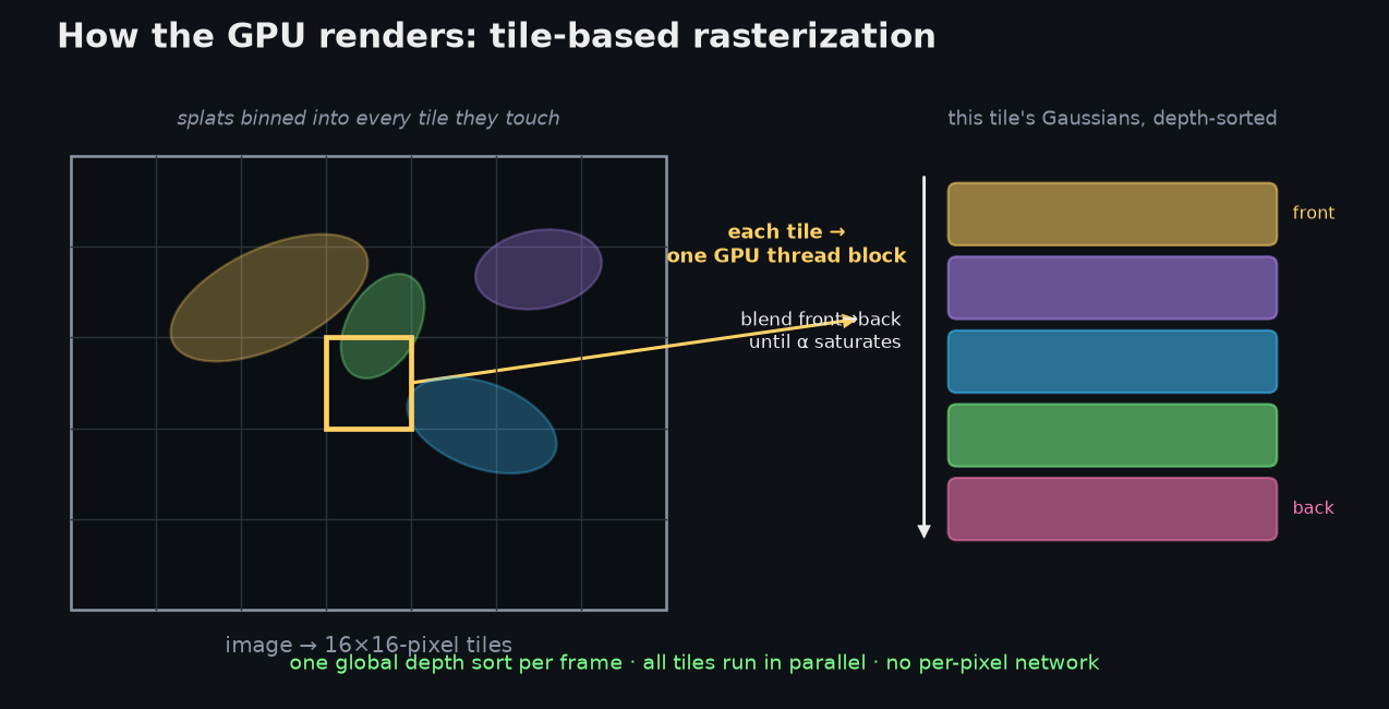
2. Bin into tiles. The frame is cut into 16×16-pixel tiles. Each Gaussian emits one entry for every tile its bounding box covers — so a big splat is duplicated across many tiles — and each entry's 64-bit sort key packs the tile ID in the high bits and the depth in the low bits.
3. One global sort. A single GPU radix sort over all those keys simultaneously groups entries by tile and orders them by depth within each tile. This is the trick that makes it fast: you sort once per frame instead of once per pixel, and all 256 pixels of a tile then share one ordered list. (The ordering is per-tile, not strictly per-pixel — a cheap approximation that can cause occasional "popping," and which the alias-free follow-ups tighten up.)
4. Blend — one thread block per tile. Each tile is handed to a block of 256 threads, one per pixel. The block cooperatively loads its sorted splats into fast shared memory in batches; each thread then walks that list front-to-back, accumulating color $C = \sum_i c_i\,\alpha_i\,T_i$ while decaying the transmittance $T \leftarrow T\,(1-\alpha_i)$, and stops early the instant its pixel saturates ($T$ near zero). Tiles are independent, so thousands run at once.

The payoff is ≥30 fps — often hundreds — at 1080p: the work is embarrassingly parallel, the depth sort is amortized over a whole frame, and the per-pixel inner loop is a handful of multiply-adds with an early-out, not a network evaluation. At inference this forward pass is the entire renderer.

Training on the GPU

Training is that same rasterizer run backwards, ~30k times. Each iteration:

1. Forward render a training viewpoint with the pipeline above, then compute the loss $\mathcal{L}$ (the L1 + D-SSIM from earlier) against the real photo — both on the GPU.
2. Backward rasterizer. A second custom CUDA kernel mirrors the forward one, walking each tile's sorted list back-to-front and turning $\partial\mathcal{L}/\partial C(p)$ into gradients for every Gaussian that touched the pixel — with respect to its color, opacity, and 2D position and covariance. To avoid caching the blend state of every splat at every pixel (which would exhaust memory), it reconstructs the weights it needs from a little stored per-pixel state as it sweeps backward. Those 2D gradients are then chained back through the projection onto the 3D mean, the scale and rotation that compose $\Sigma$, and the SH coefficients. Because one splat lands in many pixels and tiles, contributions are summed with atomic adds.
3. Optimizer step. Adam updates the parameters of all Gaussians at once — and there are a lot of them: position (3), scale (3), a rotation quaternion (4), opacity (1), and SH color (48 at degree 3) ≈ 59 numbers per Gaussian, times millions of Gaussians, every step.
4. Adaptive density control (every few hundred steps) is the part unique to splatting, and it runs off the gradients you just computed:

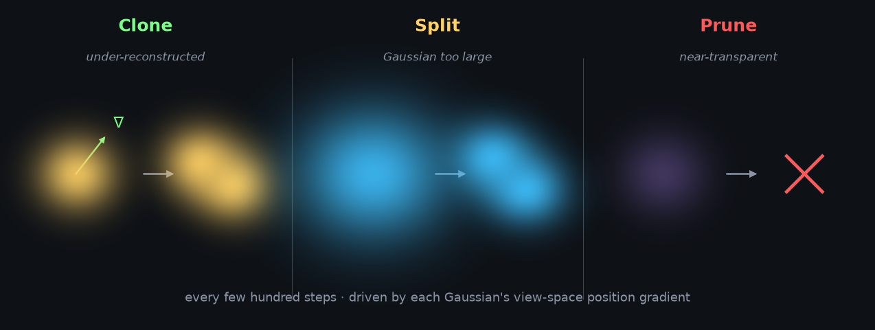
• Clone — where the view-space position gradient is large but the Gaussians there are small, the region is under-reconstructed, so small Gaussians are duplicated and nudged along the gradient to add coverage.
• Split — where a single Gaussian has grown too large (over-reconstructed), it's replaced by two smaller ones (scale divided by ≈1.6), with positions sampled from the original's own distribution.
• Prune — Gaussians whose opacity has decayed below a threshold are deleted, and opacities are periodically reset to flush out floaters.

These are all parallel operations over the parameter buffers (plus a compaction), so the Gaussian count grows and shrinks mid-training without stalling the GPU.

Because a forward-plus-backward pass is only milliseconds, tens of thousands of steps finish a scene in roughly 30–60 minutes on a single consumer GPU (a 3090/4090-class card). The hard ceiling is VRAM: every explicit Gaussian and its ~59 parameters live in GPU memory, which is exactly why the compression work below matters — and why scaling to genuinely huge scenes means sharding the Gaussians across multiple GPUs.

A closer look at the CUDA kernels

It's worth opening the hood, because the whole thing is a surprisingly small stack of CUDA kernels glued together with two library primitives. Here's where the data lives and what runs in parallel:

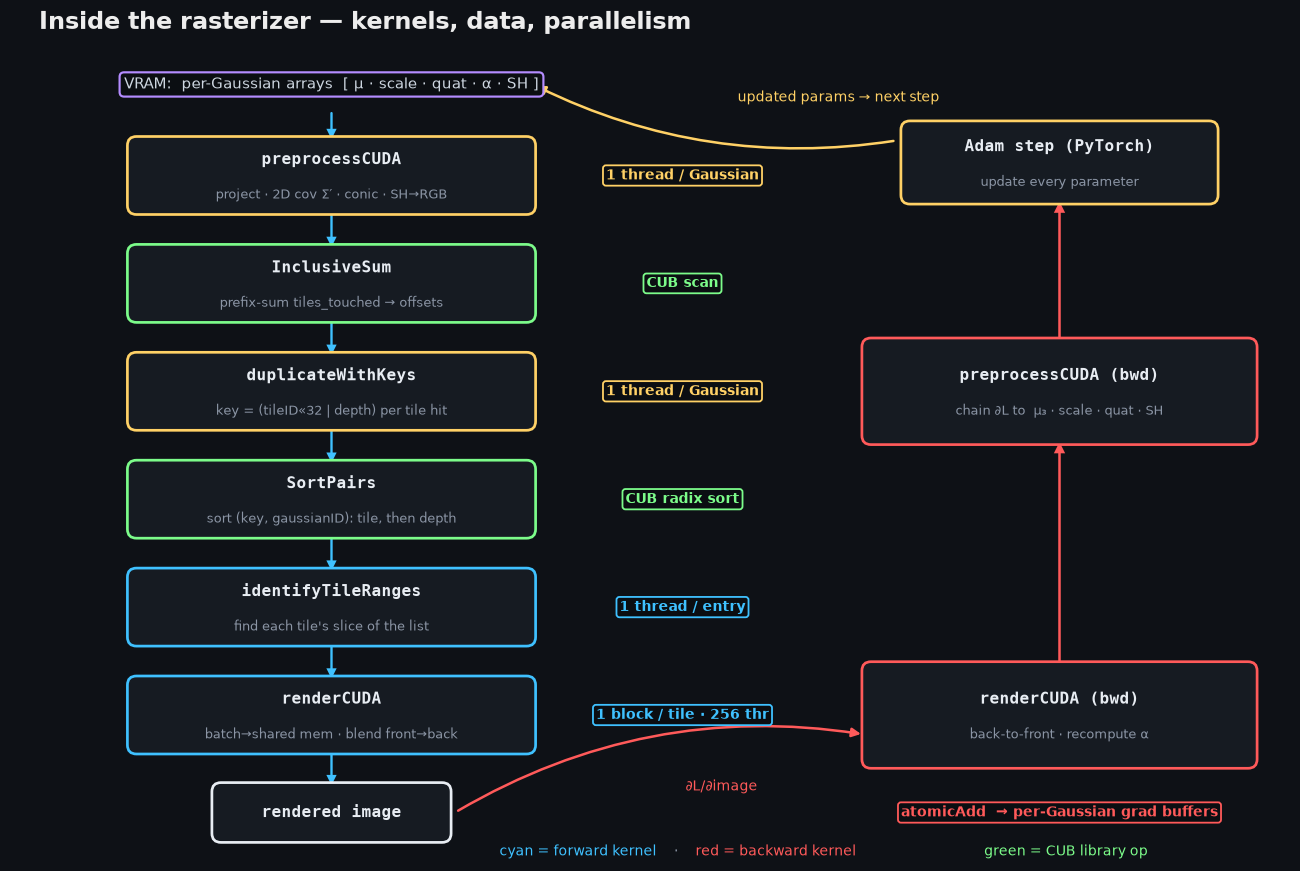
The data is a handful of flat per-Gaussian arrays in VRAM — means, scales, rotation quaternions, opacities, SH coefficients — laid out struct-of-arrays so threads read them coalesced. Training keeps a matching set of gradient buffers of the same shape.

The forward pass is six kernels (left column above). Two distinct kinds of parallelism show up, and which one a stage uses is the thing to notice:

• preprocessCUDA — one thread per Gaussian. Projects the mean, forms the 2D covariance and its inverse (the "conic"), evaluates SH → RGB for this view, and counts how many 16×16 tiles the splat covers.
• InclusiveSum — a CUB device-wide prefix scan over tiles_touched, which hands each Gaussian the offset where its keys go in one big list.
• duplicateWithKeys — one thread per Gaussian. For every tile a splat touches, it writes a 64-bit key (tileID << 32 | depth) and the Gaussian's id.
• SortPairs — a CUB device-wide radix sort of those (key, id) pairs. Packing the tile in the high bits and depth in the low bits means a single sort groups by tile and orders by depth at once.
• identifyTileRanges — one thread per list entry. Marks where each tile's slice of the sorted list begins and ends.
• renderCUDA — one thread block per tile (16×16 = 256 threads, one per pixel). The block cooperatively streams its Gaussians through shared memory in batches of 256, and each thread blends front-to-back with an early-out.

The backward pass is two kernels (right column), run in the opposite order:

• renderCUDA (backward) — same per-tile blocks, but it walks each tile's list back-to-front, recomputing each α on the fly, and scatters gradients with atomicAdd into the per-Gaussian buffers (a single splat is hit by many pixels, so the adds must be atomic).
• preprocessCUDA (backward) — one thread per Gaussian again, chaining those 2D gradients back through the projection and SH to ∂L/∂mean₃, ∂L/∂scale, ∂L/∂quaternion, and ∂L/∂SH.

Then Adam (in PyTorch) consumes those gradient buffers and writes the parameters back, closing the loop. Sketched, the heart of it is just:

// FORWARD preprocess — one thread per Gaussian
int i = blockIdx.x * blockDim.x + threadIdx.x;        // a Gaussian
float2 xy    = project(means3D[i], view, proj);
float3 cov2D = computeCov2D(means3D[i], scales[i], rots[i], view);  // J·W·Σ·Wᵀ·Jᵀ
conic[i]     = invert(cov2D);
rgb[i]       = shToColor(sh[i], campos - means3D[i]);
tiles_touched[i] = tilesCovered(xy, radius(cov2D));

// two library primitives do the heavy lifting:
cub::DeviceScan::InclusiveSum(tiles_touched, offsets, P);
cub::DeviceRadixSort::SortPairs(keys, gaussian_ids, N);   // key = tile<<32 | depth

// FORWARD render — one BLOCK per tile, 256 threads (one per pixel)
__shared__ float2 s_xy[256];
__shared__ float4 s_conic_op[256];                    // conic + opacity
float  T = 1.0f; float3 C = make_float3(0,0,0);
for (int base = range.x; base < range.y; base += 256) {
    s_xy[tid]       = points_xy[ ids[base + tid] ];   // coalesced load to shared mem
    s_conic_op[tid] = conic_opacity[ ids[base + tid] ];
    __syncthreads();
    for (int j = 0; j < 256 && !done; ++j) {          // front -> back
        float a = s_conic_op[j].w * expf(power(s_xy[j], pixel));
        C += rgb[j] * (a * T);  T *= (1.0f - a);
        if (T < 1e-4f) done = true;                   // early termination
    }
}

// BACKWARD render — same tiling, back-to-front, gradients via atomics
atomicAdd(&dL_dmean2D[g],  ...);  atomicAdd(&dL_dconic[g],    ...);
atomicAdd(&dL_dopacity[g], ...);  atomicAdd(&dL_dcolor[g][c], ...);

So the operators that actually matter are a CUB scan, a CUB radix sort, and a lot of atomicAdd over shared-memory-tiled blocks — no general-purpose autodiff graph, no locks. That's the engineering reason a scene trains in minutes rather than hours. (The snippet is sketched for shape, not the verbatim reference kernels.)

Why Gaussians, and not points or triangles?

This was my nagging question — why this primitive? It's because a Gaussian sits in exactly the right spot between the alternatives:

• A point has no extent. You'd need an impossible number of them, and there's nothing to interpolate between samples.
• A triangle needs explicit surface topology — you have to decide, up front, which points connect to which, and that's the hard, brittle part of meshing.
• A Gaussian is point-like enough to be flexible, surface-like enough to render smooth shapes when you flatten it, and volumetric enough to model fuzzy, uncertain, semi-transparent regions when you don't.

Real photo reconstruction is messy, and the Gaussian lets you stay non-committal about geometry while still rendering something that looks right. You never have to declare "this is a surface and here is its mesh."

Why it became so popular

Put it together and you can see why it spread so fast:

• Fast to train relative to classic NeRF — you're optimizing explicit particles, not distilling everything into an opaque network.
• Real-time to render — projecting splats maps onto the GPU rasterization pipeline instead of ray-marching a dense field. The original work leaned hard on ≥30 fps at 1080p.
• Photorealistic from ordinary captures — phone video of a cluttered real scene, leaves and wires and all.
• Editable-ish — because it's explicit blobs in space, you can inspect, move, segment, prune, compress, or combine them far more naturally than you can edit a neural field.
• A great fit for AR/VR and spatial computing — a compact, renderable scene straight from a capture, which is why people started calling it a "JPEG moment" for scanned environments.

Where it falls down

It's not magic, and the limitations are real:

• It's not a clean mesh. You get a gorgeous visual representation, not usable geometry. Collision, physics, relighting, and CAD-style editing are all harder than with a normal mesh.
• Memory is heavy. Millions of Gaussians, each with position, covariance, opacity, and SH color, add up fast. Compression is an active front — Niedermayr et al. report up to 31× compression with minimal visual loss using vector clustering and quantization-aware training.
• View extrapolation is limited. It's excellent near the captured camera trajectory and starts revealing holes, floaters, and hallucinated detail when you wander somewhere no photo ever saw. (You can see exactly those floaters as stray blobs in the training video above.)
• Geometry can be wrong even when the image looks right. Vanilla 3DGS optimizes for view synthesis, not surface accuracy, which is what motivated 2D Gaussian Splatting — collapsing each blob into an oriented planar disk to get view-consistent surfaces.
• Aliasing under scale changes. Zoom in or change focal length and you get artifacts; Mip-Splatting added a 3D smoothing filter and a 2D Mip filter to keep rendering alias-free.

That last cluster of follow-up papers is the tell that this is a young, fast-moving representation. But the core idea is one of those things that feels obvious in hindsight: if you're going to optimize a scene against photos with a differentiable renderer, don't hide it inside a neural network — lay it out explicitly as a million soft blobs, and let the GPU do what it's good at.